
Infrastructure Self-Calibration for radio-based indoor positioning

Radio positioning needs the positions of its anchors, access points, base stations, or reconfigurable intelligent surfaces, and manual surveying is costly and error-prone. Calibrating this infrastructure from its own measurements is one estimation problem, studied in at least four communities as self-calibration, auto-positioning, anchor self-localization, network localization, or radio simultaneous localization and mapping (SLAM).

This page collects five works on the problem, from a Bayesian grid filter in 2022 to a tutorial with reference implementations and an open ultra-wideband (UWB) dataset in 2026. The tutorial teaches the problem through one factor graph, in which the measurement topology sets the factors and the reference information enters as priors.

Tutorial preprint Code: radiocal Dataset: UWB-ASC

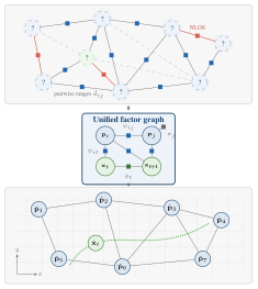
Three stacked panels. Top: anchors of unknown position, each marked with a question mark, linked by range measurements, some of them non-line-of-sight and some out of range, with a mobile tag in green. Middle: the unified factor graph, with anchor variables, two tag poses, and range, motion and prior factors. Bottom: the calibrated anchor map with the estimated tag path.
From ranges among anchors of unknown position (?) and a mobile tag, through one factor graph, to the calibrated anchors and the path of the tag. Tutorial, Fig. 1.

One operation, twenty names

20

title terms across the 36 papers of the terminology review, most of them used by a single paper

1

operation: estimating the positions of static reference points from range measurements, without manual surveying

No term has prevailed. The review recommends self-calibration as the canonical process term and anchor as the default entity prefix, reflecting the UWB-dominant corpus. More on the review

Four measurement topologies

The measurement topology is the set of node pairs that measure ranges. Four topologies recur across the literature under otherwise unrelated names, and the tutorial draws each as a factor graph.

Legend: anchor p_i as a blue circle, pose x_t as a green circle, range factor psi as a black square, motion factor phi as a green square, and a dashed line for out of range.
The four measurement topologies as factor graphs. Tutorial, Fig. 3.

From deployment to method

The tutorial draws three lessons from its examples on the two deployments of UWB-ASC, one with line-of-sight (LOS) and one rich in non-line-of-sight (NLOS) propagation. Its decision tree combines them with the theory of the tutorial into a choice of method.

The examples cover two-dimensional UWB two-way ranging at the two deployments and one public scan, so the lessons are demonstrations within that scope.

Decision tree

Which method fits your deployment? Answer a few short questions about it. They concern only the deployment and can be answered before any algorithm is chosen, and the last step names a topology, a method and the examples behind it. Before the first question, the tree adds the nuisance states of the measurement primitive (Table IV). Section and table numbers refer to the tutorial.

The whole tree as a figure
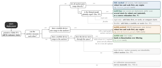
Decision tree. Start at the deployment and add the nuisance states of its primitive. If the anchors can measure each other and a mobile device also ranges to them, the leaf is mobile-assisted. If no mobile device ranges and all anchor pairs range directly, the leaf is fully meshed. Otherwise the thinned graph is tested for global rigidity, which leads to the multi-hop leaf, or to adding links, a mobile or seeds, or to comparing starts. If the anchors cannot measure each other, a moving device leads to the mobile-only leaf, a static device to collecting motion, and no calibration measurements to a manual survey.
Decision tree from the primitive and edge set of a deployment to a topology and an algorithm family. Leaves name their evidence in Section VI. Tutorial, Fig. 12.

Research

  1. Bayesian grid filter at IPIN
  2. NLOS recordings of UWB-ASC
  3. LOS recordings of UWB-ASC
  4. Terminology review in IEEE Access
  5. Uncertainty propagation in IEEE JISPIN
  6. UWB-ASC 1.0.0 and descriptor
  7. Tutorial preprint and radiocal 1.0.0

PreprintUnder review · 2026

A Tutorial on Infrastructure Self-Calibration for Radio-Based Indoor Positioning

Paul Schwarzbach

Teaches infrastructure self-calibration as one factor graph and carries a recorded session through every step, with released code that recomputes every result table.

Aim. To let a reader state a deployment as one factor graph, judge from its edge set what the ranges can identify, choose an algorithm family and its starting point, and check a calibration before trusting it.

Two-dimensional UWB two-way ranging. One static session of the LOS deployment of UWB-ASC runs through every step, and the NLOS deployment and the public TWR-CLOUD-Bern dataset serve as contrasts.

  • Range-based calibration is one factor graph. The measurement topology sets its factors, and the reference information enters as priors.
  • Rigidity and the motion of a mobile device decide what the ranges can identify. Multidimensional scaling, nonlinear least squares, recursive filters and convex relaxations act as inference engines over the same graph and differ in their data interface and in their need for a starting point.
  • Three lessons and a decision tree lead from a deployment to a method, and the released code recomputes every result table.
Anchor RMSE without and with the action of each finding. Tutorial, Table VI.
Finding and actionWherewithout (m)with (m)
Loss before engine (VI-A): gaussian → cauchyfull meshes, NLOS deployment3.940.79
Start decides (VI-B): classical start → oracle startglobally rigid random views of s034.030.24
Range bias (VI-C): no offsets → per-device offsetsfull meshes, LOS deployment0.230.13
Mobile-only (VI-D): ekf_slam → fg_slamwalk s01, LOS deployment1.880.36
Seeds (VI-E): blind → three seedsκ=3 view of s030.430.71

Aligned anchor RMSE of the factor graph or of the engines a row names, under the cauchy kernel unless the action changes it, as medians where a row covers several sessions or views. The oracle start is the survey, and κ is the thinning level of the multi-hop views.
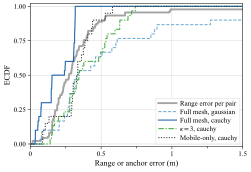
Empirical distribution functions for the LOS deployment: the range error per anchor pair, and the anchor errors of the factor graph on the full mesh with the gaussian and the cauchy kernel, on the multi-hop view with kappa 3, and on the mobile-only view. The cauchy full-mesh curve rises steepest.
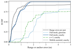
Empirical distribution functions for the NLOS deployment, on its own clipped abscissa: the range error per anchor pair, and the anchor errors of the factor graph on the full mesh with the gaussian and the cauchy kernel, on the multi-hop view with kappa 3, and on the mobile-assisted view. The gaussian full-mesh curve rises last.
Empirical cumulative distribution functions (ECDF) of the absolute session-median range residual per anchor pair and of the aligned error per anchor of the factor graph, pooled over the sessions. Each panel clips its own abscissa. Tutorial, Fig. 8.

IEEE JISPINVol. 4, pp. 161–170, 2026 · open access

Evaluation of Grid-Based Uncertainty Propagation for Collaborative Self-Calibration in Indoor Positioning Systems

Paul Schwarzbach, Andrea Jung (equal contribution)

On measured UWB ranges, propagating the position uncertainty of the anchors through a grid loses little accuracy when NLOS links enter the initialization, unlike a closed-form method.

Question. Does grid-based uncertainty propagation keep the collaborative self-calibration of a UWB network accurate on measured ranges in a mixed LOS and NLOS environment, also when NLOS links enter its initialization?

12 UWB nodes ranging as a full mesh in an industrial hall, with total-station ground truth. The static sessions of the NLOS deployment of UWB-ASC served this study. The paper extends the grid-based Bayesian formulation of the IPIN 2022 paper.

  • Under LOS initialization the probabilistic grid-based positioning (PGP) reaches median errors of 0.34–0.68 m, with 66–92% of the estimates below 1 m.
  • With NLOS links in the initialization triangle, PGP keeps median errors of 0.62–0.99 m. The closed-form (CF) baseline reaches median errors of 1.48–2.43 m, with outliers beyond 30 m.
  • PGP keeps full positioning availability whatever the initialization, while the availability of single nodes under the CF baseline drops to zero or a few percent in some configurations.
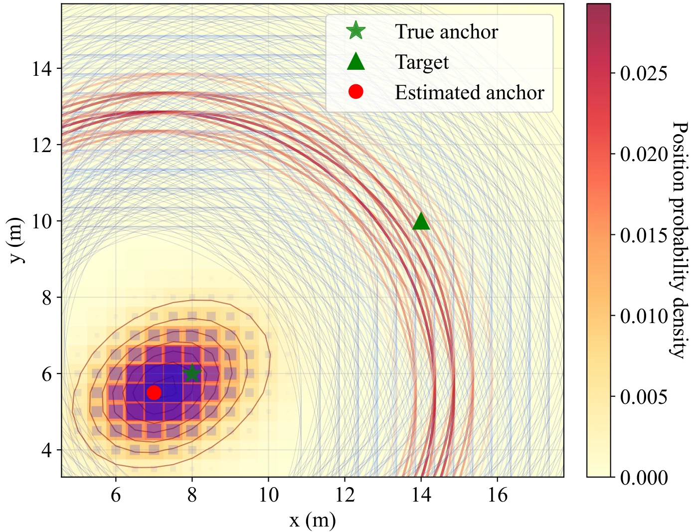
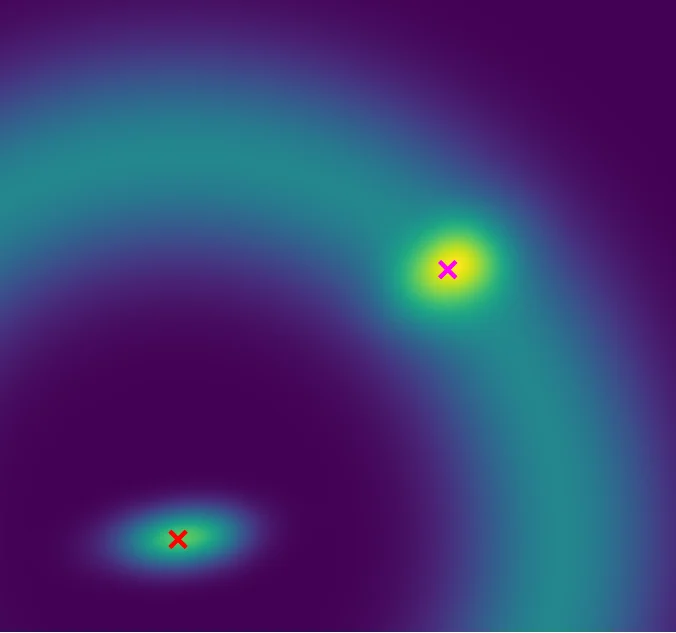
Probability grid of an anchor position near the lower left, with the true anchor as a green star and the estimate as a red dot. Weighted range circles radiate from the grid cells towards a target, drawn as a green triangle, instead of a single circle from a point estimate. A colour bar gives the position probability density.
Grid-based uncertainty propagation for collaborative self-calibration: Anchor probability distribution generates multiple weighted measurement hypotheses (radiating lines) rather than single point-estimate constraints, preserving spatial uncertainty information for reliable localization. JISPIN paper, Fig. 1, CC BY 4.0.
Positioning error across four initialization configurations, three of the columns of Table III of the paper. Conf. 1 and 2 start from line-of-sight triangles, Conf. 3 and 4 from triangles with two NLOS links of three.
ConfigurationMethodMedian (m)p95 (m)below 1 m (%)
Conf. 1 (LOS)PGP0.682.0066.1
CF0.477.5977.2
Conf. 2 (LOS)PGP0.341.1291.6
CF0.401.8479.4
Conf. 3 (NLOS)PGP0.622.0573.3
CF2.437.1829.9
Conf. 4 (NLOS)PGP0.992.5450.3
CF1.4830.3545.2

IEEE AccessVol. 14, pp. 51603–51619, 2026 · open access

Terminology Fragmentation of Infrastructure Calibration in Radio-Based Indoor Positioning: A Systematic Review

Paul Schwarzbach

A systematic review finds 20 title terms for one operation in 36 papers and recommends self-calibration as the canonical term.

Questions. What namespace inconsistencies exist for autonomous reference point surveying across technology domains, and how has the terminology evolved from 2015 to 2025?

A systematic review following the Preferred Reporting Items for Systematic Reviews and Meta-Analyses (PRISMA). Its search covers four databases from 2015 to 2025, screening 461 deduplicated records and analyzing 36 included papers.

  • The 36 papers use 20 distinct title-level terms for a single operation, with a 70% singleton rate, and 137 unique variants in their full texts. UWB accounts for 31 of the 36 papers.
  • No convergence has occurred. The share of papers using self-calibration declined from 100% (2015–2017) to 22% (2022–2026) as competing terms proliferated.
  • The review recommends self-calibration as the canonical process term and anchor as the default entity prefix, reflecting the UWB-dominant corpus. Technology-appropriate alternatives such as access point or beacon are equally valid.
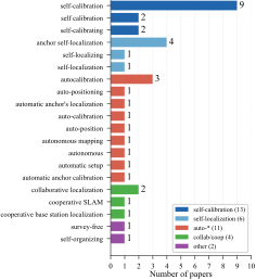
Horizontal bar chart of the 20 primary title-level terms across the 36 included papers, coloured by prefix family. Self-calibration leads with 9 papers, anchor self-localization follows with 4 and autocalibration with 3, and most other terms occur once. The legend counts 13 papers for the self-calibration family, 6 for self-localization, 11 for auto-star, 4 for collaborative or cooperative, and 2 for other.
Primary title-level terms across 36 included papers. Terms are grouped and color-coded by prefix family. IEEE Access paper, Fig. 4, CC BY 4.0.

IPIN 202212th International Conference on Indoor Positioning and Indoor Navigation, 5–7 September 2022, Beijing

Auto-Positioning in Radio-based Localization Systems: A Bayesian Approach

Andrea Jung, Paul Schwarzbach, Oliver Michler

In simulation, a Bayesian grid filter that propagates the position uncertainties of all nodes reaches a higher positioning accuracy than a closed-form approach.

Question. Can a discrete Bayesian method that propagates the position uncertainties of all nodes make auto-positioning robust to multipath errors, outliers and measurement failures, and lower its demands on the availability of observations, compared with a closed-form approach?

Simulated ranges among 13 nodes, 1,000 epochs per scenario, in three scenarios from LOS noise only to frequent outliers.

  • The collaborative grid positioning (CGP), a multi-dimensional histogram filter, reaches at least 58% higher positioning accuracy than the closed-form baseline.
  • With Gaussian LOS ranges, the node RMSE is 0.17 m for CGP against 0.41 m for the closed form.
  • With multipath errors, outliers and measurement failures in scenario III, the RMSE is 0.93 m for CGP against 6.99 m for the closed form.
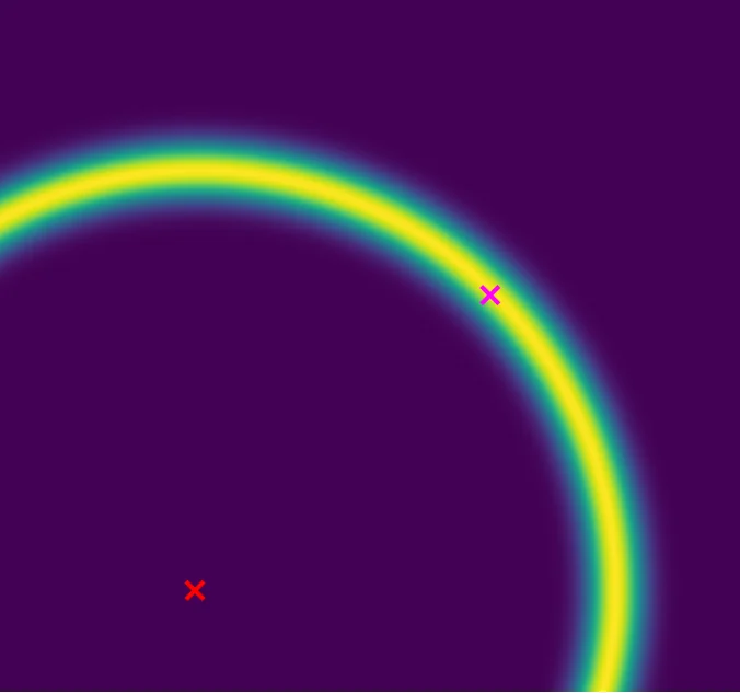
Heat map of the observation likelihood for a stationary reference node: a sharp ring at the measured range around the node.(a) Stationary
Heat map of the observation likelihood for a non-stationary reference node: the ring widens, since the position uncertainty of the reference node enters the likelihood.(b) Non-stationary
Observation variance: (a) uncorrelated case with stationary nodes, (b) correlated case for non-stationary nodes. IPIN 2022 paper, Fig. 5, © 2022 IEEE.

Dataset: UWB-ASC

LOS deployment set_b

UWB-ASC, LOS deployment, layout from the survey and the field labels Surveyed nodes, control points and pairs labeled NLOS of the LOS deployment of UWB-ASC 1.0.0 in its own survey frame, with the logged tag poses of the walks s01 and s02. The node table beside the map lists the same positions. Logged tag poses of the walks s01 and s02 (DD98, motion capture), every third pose 4197–4AA4 · pair labeled NLOS 4197–D5B4 · pair labeled NLOS 4503–5BB6 · pair labeled NLOS 4A23–5BB6 · pair labeled NLOS 4AA4–5388 · pair labeled NLOS 4AA4–9911 · pair labeled NLOS 5388–5BB6 · pair labeled NLOS 5BB6–8B05 · pair labeled NLOS 5BB6–D38F · pair labeled NLOS 8AA5–D5B4 · pair labeled NLOS 8B05–D5B4 · pair labeled NLOS 9911–D5B4 · pair labeled NLOS D38F–D5B4 · pair labeled NLOS GCP-11 · control or reference point · x 31.15 m, y 45.71 mGCP-08 · control or reference point · x 20.50 m, y 57.39 mGCP-13 · control or reference point · x 27.80 m, y 60.76 m3 · control or reference point · x 32.41 m, y 50.71 mWAND-0-0 · origin of the Vicon frame · x 26.87 m, y 53.63 m 4197 · anchor · x 28.35 m, y 61.45 m4503 · anchor · x 26.79 m, y 46.94 m4A23 · anchor of the prior subset · x 34.11 m, y 51.73 m4AA4 · anchor · x 22.47 m, y 43.48 m5388 · anchor · x 23.92 m, y 45.62 m5BB6 · anchor of the prior subset · x 19.15 m, y 41.33 m8AA5 · anchor · x 20.98 m, y 47.48 m8B05 · anchor of the prior subset · x 21.23 m, y 56.50 m9911 · anchor · x 30.90 m, y 58.13 mD38F · anchor · x 18.36 m, y 54.84 mD5B4 · surveyed node that never ranges · x 17.48 m, y 45.14 m

NLOS deployment set_a

UWB-ASC, NLOS deployment, layout from the survey and the field labels Surveyed nodes, control points and pairs labeled NLOS of the NLOS deployment of UWB-ASC 1.0.0 in its own survey frame, with the markers of the roving tag of the quasi-static sessions s01 to s20. The node table beside the map lists the same positions. 4197–D5B4 · pair labeled NLOS 4503–5388 · pair labeled NLOS 4503–8AA5 · pair labeled NLOS 4503–D5B4 · pair labeled NLOS 4A23–8AA5 · pair labeled NLOS 4AA4–5388 · pair labeled NLOS 4AA4–8AA5 · pair labeled NLOS 4AA4–D5B4 · pair labeled NLOS 5388–5BB6 · pair labeled NLOS 5388–8B05 · pair labeled NLOS 5388–9911 · pair labeled NLOS 5388–D38F · pair labeled NLOS 5BB6–8AA5 · pair labeled NLOS 5BB6–D5B4 · pair labeled NLOS 8AA5–9911 · pair labeled NLOS 8AA5–D38F · pair labeled NLOS 8AA5–DD98 · pair labeled NLOS 8B05–D5B4 · pair labeled NLOS 9911–D5B4 · pair labeled NLOS D38F–D5B4 · pair labeled NLOS REFP01 · control or reference point · x 7.60 m, y 8.14 mREFP02 · control or reference point · x 6.72 m, y 0.13 mREFP03 · control or reference point · x 13.15 m, y -1.42 m 4197 · anchor · x 8.18 m, y -3.58 m4503 · anchor · x 7.88 m, y 12.03 m4A23 · anchor of the prior subset · x -3.47 m, y -3.95 m4AA4 · anchor · x -26.99 m, y 3.37 m5388 · anchor · x -7.42 m, y 23.17 m5BB6 · anchor of the prior subset · x -27.37 m, y -4.10 m8AA5 · anchor · x -15.15 m, y 19.14 m8B05 · anchor of the prior subset · roving tag of the sessions s01 to s20 · x 7.49 m, y 4.16 m9911 · anchor · x -27.95 m, y 11.17 mD38F · anchor · x -12.01 m, y 11.11 mD5B4 · anchor · x -2.21 m, y 23.28 mDD98 · anchor · x -12.35 m, y -4.11 m P01 · marker of the roving tag · session s01 · x 7.54 m, y 4.16 mP02 · marker of the roving tag · session s02 · x 4.69 m, y 4.13 mP03 · marker of the roving tag · session s03 · x 3.31 m, y 1.88 mP04 · marker of the roving tag · session s04 · x 3.44 m, y -2.06 mP05 · marker of the roving tag · session s05 · x -0.08 m, y -3.67 mP06 · marker of the roving tag · session s06 · x -3.48 m, y 1.40 mP07 · marker of the roving tag · session s07 · x -3.59 m, y 7.77 mP08 · marker of the roving tag · session s08 · x -3.40 m, y 11.99 mP09 · marker of the roving tag · session s09 · x -3.39 m, y 17.53 mP10 · marker of the roving tag · session s10 · x -6.33 m, y 21.80 mP11 · marker of the roving tag · session s11 · x -11.79 m, y 16.93 mP12 · marker of the roving tag · session s12 · x -13.35 m, y 21.26 mP13 · marker of the roving tag · session s13 · x -12.82 m, y 7.76 mP14 · marker of the roving tag · session s14 · x -16.17 m, y 2.77 mP15 · marker of the roving tag · session s15 · x -19.02 m, y -3.36 mP16 · marker of the roving tag · session s16 · x -24.20 m, y -3.26 mP17 · marker of the roving tag · session s17 · x -20.77 m, y 3.66 mP18 · marker of the roving tag · session s18 · x -25.30 m, y 8.06 mP19 · marker of the roving tag · session s19 · x -19.38 m, y 12.32 mP20 · marker of the roving tag · session s20 · x 4.94 m, y 10.07 m
Layout of both deployments. Interactive form of descriptor Fig. 2, drawn from the files of UWB-ASC 1.0.0.

Anchor self-calibration estimates the positions of fixed nodes of an indoor radio positioning or localization system from observations among the nodes and to mobile devices. The UWB Anchor Self-Calibration Dataset (UWB-ASC) is a testing ground for such methods, recorded in one industrial hall in Torgau, Germany, with UWB two-way ranging.

In the LOS deployment, 10 anchors range with a walking tag tracked by motion capture. In the NLOS deployment, 12 nodes range among obstructions, and one of them roves over surveyed markers in 20 quasi-static sessions. Both deployments also hold static sessions, and a total station surveyed every fixed node.

The HYMN multi-technology dataset comes from the same hall, and its project page shows photos of the hall.

Each panel shows one deployment in its own survey frame, drawn from the survey and the field labels, and the LOS panel adds the logged tag poses of the walks s01 and s02. Pointing at a mark shows its identifier and position.

  • anchor
  • anchor of the prior subset
  • surveyed node that never ranges
  • control or reference point
  • marker of the roving tag
  • origin of the Vicon frame
  • logged tag pose
  • pair labeled NLOS
Node positions as a table
LOS deployment (set_b): surveyed positions from Data/set_b/nodes.yaml of UWB-ASC 1.0.0, in the survey frame of the deployment.
IdShown asx (m)y (m)z (m)
4A23anchor of the prior subset34.11251.7344.557
5BB6anchor of the prior subset19.14741.3334.553
8B05anchor of the prior subset21.22556.4974.569
4197anchor28.35161.4534.567
4503anchor26.78546.9384.556
4AA4anchor22.46743.4814.553
5388anchor23.91645.6184.577
8AA5anchor20.98447.4764.557
9911anchor30.90358.1334.563
D38Fanchor18.35554.8394.537
D5B4surveyed node that never ranges17.47645.1364.553
3control or reference point32.41450.7063.059
GCP-08control or reference point20.50157.3892.945
GCP-11control or reference point31.15345.7141.859
GCP-13control or reference point27.80560.7572.936
WAND-0-0origin of the Vicon frame26.87153.6302.927
NLOS deployment (set_a): surveyed positions from Data/set_a/nodes.yaml of UWB-ASC 1.0.0, in the survey frame of the deployment.
IdShown asx (m)y (m)z (m)
4A23anchor of the prior subset-3.473-3.9501.252
5BB6anchor of the prior subset-27.373-4.1021.289
8B05anchor of the prior subset7.4884.1601.310
4197anchor8.179-3.5791.301
4503anchor7.87512.0341.337
4AA4anchor-26.9913.3681.293
5388anchor-7.42123.1691.312
8AA5anchor-15.15319.1451.312
9911anchor-27.94511.1671.307
D38Fanchor-12.01211.1051.262
D5B4anchor-2.20823.2791.234
DD98anchor-12.352-4.1051.266
P01marker of the roving tag7.5424.161-0.409
P02marker of the roving tag4.6904.131-0.431
P03marker of the roving tag3.3141.878-0.431
P04marker of the roving tag3.440-2.061-0.448
P05marker of the roving tag-0.080-3.670-0.438
P06marker of the roving tag-3.4851.398-0.438
P07marker of the roving tag-3.5887.768-0.428
P08marker of the roving tag-3.40311.990-0.444
P09marker of the roving tag-3.38917.533-0.459
P10marker of the roving tag-6.33121.802-0.425
P11marker of the roving tag-11.79216.931-0.443
P12marker of the roving tag-13.34621.257-0.424
P13marker of the roving tag-12.8217.756-0.435
P14marker of the roving tag-16.1712.765-0.430
P15marker of the roving tag-19.021-3.357-0.437
P16marker of the roving tag-24.205-3.263-0.434
P17marker of the roving tag-20.7663.661-0.424
P18marker of the roving tag-25.2958.060-0.433
P19marker of the roving tag-19.37712.316-0.452
P20marker of the roving tag4.94410.069-0.447
REFP01control or reference point7.6028.137-0.419
REFP02control or reference point6.7240.133-0.418
REFP03control or reference point13.148-1.417-1.562

Descriptor Zenodo GitHub

The descriptor (Paul Schwarzbach, arXiv:2611.11579) is submitted to IEEE Data Descriptions.

Contents

Measured deployments
Static, quasi-static and walking sessions on one node set under LOS and NLOS propagation, with the surveyed nodes and the motion-capture truth of the walks.
Range simulator
A seeded range simulator draws synthetic ranges on the surveyed geometry with adjustable error components, from noise-free ranges to NLOS errors. Its 81 frozen draws in 5 conditions serve as the reference.
Readers of public data
Readers convert the ranges among the static nodes of two public UWB datasets, TWR-CLOUD-Bern and selfloc, into the same format without redistribution.
Formats
All parts share open Parquet and YAML files, in which topology views select the ranges for each class of calibration method. Raw recordings with rebuild scripts, quality reports and field labels of the line of sight complete the dataset.

Scope and limits

  • One hall and one hardware family, the modules of a Qorvo MDEK1001 development kit with the DW1000 chip, whose physical-layer settings were not recorded.
  • The anchors stand at nearly one height, so both layouts are close to planar.
  • No inertial measurements and no channel impulse responses.
  • Untested uses include three-dimensional calibration, methods that fuse inertial data or channel features, and the transfer to other chip generations.

Quick start

Python 3.10 or newer, no GPU. Install from the repository root and run the smoke test:

git clone https://github.com/PaulSchwarzbach/UWB-ASC-dataset
cd UWB-ASC-dataset
pip install -e "Code/datasets/radiocal[qa,methods]"
python -B tests/test_smoke.py

One session in a few lines:

import radiocal

g = radiocal.load_session("Data/set_b/s01")   # superset graph of one session
view = g.apply_mask("fully_meshed")            # anchor-anchor ranges, no priors
view.edges.head()                              # t, t_raw, seq, from_id, to_id, range_m
g.nodes                                        # id, role, prior_type, x, y, z, sigma_m

Code & data

Archived artifacts with persistent identifiers.
ArtifactArchiveSourceLicence
radiocal 1.0.0reference implementations, result tables, literature record 10.5281/zenodo.24134343 PaulSchwarzbach/radiocal code MIT, data and result tables CC BY 4.0
UWB-ASC 1.0.0sessions, range simulator, readers of public data 10.5281/zenodo.24055896 PaulSchwarzbach/UWB-ASC-dataset data CC BY 4.0, code MIT

Version DOIs. The concept DOIs 10.5281/zenodo.24134342 (radiocal) and 10.5281/zenodo.24055895 (UWB-ASC) resolve to the latest version.

radiocal in a few lines

Python 3.10 or newer, no GPU. The release holds the reference implementations with their driver, the result tables, the record of the literature search of the tutorial, and a copy of the measured sessions of UWB-ASC.

git clone https://github.com/PaulSchwarzbach/radiocal.git
cd radiocal
pip install -e "Code/datasets/radiocal[qa,methods]"
import radiocal

g = radiocal.load_session("Data/set_b/s01")   # superset graph
view = g.apply_mask("slam_bipartite")          # mobile-only view

view.edges           # DataFrame: t, t_raw, seq, from_id, to_id, range_m
view.nodes           # DataFrame: id, role, prior_type, x, y, z, sigma_m
view.symmetrized()   # undirected ranges
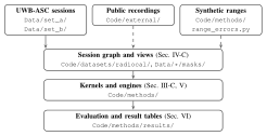
Structure of the release: the UWB-ASC sessions, public recordings and synthetic ranges feed the session graph and its views, which feed the kernels and engines, which feed the evaluation and the result tables. Each box names its folder, and the three lower boxes name the section of the tutorial that explains them.
Structure of the release, with the folder of each part and the section that explains it. Dashed inputs are not stored under Data/. Tutorial, Fig. 13.

Cite

If you use the tutorial or its code, please cite the tutorial and radiocal. If you use the data, please cite the dataset record and its descriptor.

@misc{schwarzbach_selfcal_tutorial_2026,
  author        = {Schwarzbach, Paul},
  title         = {A Tutorial on Infrastructure Self-Calibration for
                   Radio-Based Indoor Positioning},
  year          = {2026},
  eprint        = {2611.15503},
  archivePrefix = {arXiv},
  primaryClass  = {eess.SP},
  doi           = {10.48550/arXiv.2611.15503},
  note          = {Under review}
}
@misc{schwarzbach_radiocal_2026,
  author    = {Schwarzbach, Paul},
  title     = {radiocal: reference implementations and result tables for
               infrastructure self-calibration},
  year      = {2026},
  publisher = {Zenodo},
  version   = {1.0.0},
  doi       = {10.5281/zenodo.24134343},
  note      = {Code and data}
}
UWB-ASC: dataset record and descriptor
@misc{schwarzbach_uwbasc_2026,
  author    = {Schwarzbach, Paul},
  title     = {{UWB} Anchor Self-Calibration Dataset ({UWB-ASC})},
  year      = {2026},
  publisher = {Zenodo},
  version   = {1.0.0},
  doi       = {10.5281/zenodo.24055896}
}
@misc{schwarzbach_uwbasc_descriptor_2026,
  author        = {Schwarzbach, Paul},
  title         = {Descriptor: {UWB} Anchor Self-Calibration Dataset ({UWB-ASC})},
  year          = {2026},
  eprint        = {2611.11579},
  archivePrefix = {arXiv},
  primaryClass  = {eess.SP},
  doi           = {10.48550/arXiv.2611.11579},
  note          = {Submitted to IEEE Data Descriptions}
}
IEEE JISPIN 2026: grid-based uncertainty propagation
@article{schwarzbach_uncertainty_2026,
  author  = {Schwarzbach, Paul and Jung, Andrea},
  title   = {Evaluation of Grid-Based Uncertainty Propagation for Collaborative
             Self-Calibration in Indoor Positioning Systems},
  journal = {IEEE Journal of Indoor and Seamless Positioning and Navigation},
  volume  = {4},
  pages   = {161--170},
  year    = {2026},
  doi     = {10.1109/JISPIN.2026.3687458}
}
IEEE Access 2026: terminology review
@article{schwarzbach_terminology_2026,
  author  = {Schwarzbach, Paul},
  title   = {Terminology Fragmentation of Infrastructure Calibration in
             Radio-Based Indoor Positioning: A Systematic Review},
  journal = {IEEE Access},
  volume  = {14},
  pages   = {51603--51619},
  year    = {2026},
  doi     = {10.1109/ACCESS.2026.3680224}
}
IPIN 2022: Bayesian auto-positioning
@inproceedings{jung_auto-positioning_2022,
  author    = {Jung, Andrea and Schwarzbach, Paul and Michler, Oliver},
  title     = {Auto-Positioning in Radio-based Localization Systems:
               A {Bayesian} Approach},
  booktitle = {2022 IEEE 12th International Conference on Indoor Positioning
               and Indoor Navigation (IPIN)},
  pages     = {1--7},
  year      = {2022},
  doi       = {10.1109/IPIN54987.2022.9917513}
}

People & acknowledgement

Authors

  • Paul Schwarzbach iD all five works
  • Andrea Jung iD IPIN 2022 and IEEE JISPIN 2026
  • Oliver Michler iD IPIN 2022

The work was carried out at TUD Dresden University of Technology.

Acknowledgement

The IPIN 2022 study was supported by the Federal Ministry for Economic Affairs and Climate Action (BMWK) on the basis of a decision by the German Bundestag. Fynn Hansen, Albrecht Michler and Andrea Jung supported the measurement campaigns of UWB-ASC. Deveritec GmbH provided the firmware that enabled the fully meshed measurements, and MRK Management Consultants GmbH provided access to the hall. UWB-ASC was done independently of any grants or awards.